\(
\newenvironment {prompt}{}{}
\newcommand {\accordion }[0]{}
\newcommand {\ungraded }[0]{}
\newcommand {\xmDefaultPreamble }[0]{xmPreamble.tex}
\newcommand {\xmDefaultPrintstyle }[0]{xmPrintstyle.sty}
\newcommand {\todo }[0]{}
\newcommand {\oiint }[0]{{\large \bigcirc }\kern -1.56em\iint }
\newcommand {\mooculus }[0]{\textsf {\textbf {MOOC}\textnormal {\textsf {ULUS}}}}
\newcommand {\tkzTabSlope }[1]{\foreach \x /\y /\z in {#1}{\node [left = 3pt] at (Z\x 1) {\scriptsize $\y $}; \node [right = 3pt] at (Z\x 1) {\scriptsize $\z $}; }}
\newcommand {\RR }[0]{\mathbb R}
\newcommand {\R }[0]{\mathbb R}
\newcommand {\N }[0]{\mathbb N}
\newcommand {\Z }[0]{\mathbb Z}
\newcommand {\sagemath }[0]{\textsf {SageMath}}
\newcommand {\d }[0]{\,d}
\newcommand {\l }[0]{\ell }
\newcommand {\ddx }[0]{\frac {d}{\d x}}
\newcommand {\zeroOverZero }[0]{\ensuremath {\boldsymbol {\tfrac {0}{0}}}}
\newcommand {\inftyOverInfty }[0]{\ensuremath {\boldsymbol {\tfrac {\infty }{\infty }}}}
\newcommand {\zeroOverInfty }[0]{\ensuremath {\boldsymbol {\tfrac {0}{\infty }}}}
\newcommand {\zeroTimesInfty }[0]{\ensuremath {\small \boldsymbol {0\cdot \infty }}}
\newcommand {\inftyMinusInfty }[0]{\ensuremath {\small \boldsymbol {\infty - \infty }}}
\newcommand {\oneToInfty }[0]{\ensuremath {\boldsymbol {1^\infty }}}
\newcommand {\zeroToZero }[0]{\ensuremath {\boldsymbol {0^0}}}
\newcommand {\inftyToZero }[0]{\ensuremath {\boldsymbol {\infty ^0}}}
\newcommand {\numOverZero }[0]{\ensuremath {\boldsymbol {\tfrac {\#}{0}}}}
\newcommand {\dfn }[0]{\textbf }
\newcommand {\unit }[0]{\mathop {}\!\mathrm }
\newcommand {\eval }[1]{\bigg [ #1 \bigg ]}
\newcommand {\seq }[1]{\left ( #1 \right )}
\newcommand {\epsilon }[0]{\varepsilon }
\newcommand {\phi }[0]{\varphi }
\newcommand {\iff }[0]{\Leftrightarrow }
\DeclareMathOperator {\arccot }{arccot}
\DeclareMathOperator {\arcsec }{arcsec}
\DeclareMathOperator {\arccsc }{arccsc}
\DeclareMathOperator {\si }{Si}
\DeclareMathOperator {\scal }{scal}
\DeclareMathOperator {\sign }{sign}
\newcommand {\arrowvec }[1]{{\overset {\rightharpoonup }{#1}}}
\newcommand {\vec }[1]{{\overset {\boldsymbol {\rightharpoonup }}{\mathbf {#1}}}\hspace {0in}}
\newcommand {\point }[1]{\left (#1\right )}
\newcommand {\pt }[1]{\mathbf {#1}}
\newcommand {\Lim }[2]{\lim _{\point {#1} \to \point {#2}}}
\DeclareMathOperator {\proj }{\mathbf {proj}}
\newcommand {\veci }[0]{{\boldsymbol {\hat {\imath }}}}
\newcommand {\vecj }[0]{{\boldsymbol {\hat {\jmath }}}}
\newcommand {\veck }[0]{{\boldsymbol {\hat {k}}}}
\newcommand {\vecl }[0]{\vec {\boldsymbol {\l }}}
\newcommand {\uvec }[1]{\mathbf {\hat {#1}}}
\newcommand {\utan }[0]{\mathbf {\hat {t}}}
\newcommand {\unormal }[0]{\mathbf {\hat {n}}}
\newcommand {\ubinormal }[0]{\mathbf {\hat {b}}}
\newcommand {\dotp }[0]{\bullet }
\newcommand {\cross }[0]{\boldsymbol \times }
\newcommand {\grad }[0]{\boldsymbol \nabla }
\newcommand {\divergence }[0]{\grad \dotp }
\newcommand {\curl }[0]{\grad \cross }
\newcommand {\lto }[0]{\mathop {\longrightarrow \,}\limits }
\newcommand {\bar }[0]{\overline }
\newcommand {\surfaceColor }[0]{violet}
\newcommand {\surfaceColorTwo }[0]{redyellow}
\newcommand {\sliceColor }[0]{greenyellow}
\newcommand {\vector }[1]{\left \langle #1\right \rangle }
\newcommand {\sectionOutcomes }[0]{}
\newcommand {\VerbMathToks }[2]{\alteqtoks {\begin {#2} #1 \end {#2}}}
\newcommand {\DeclareMicrotypeVariants }[1]{}
\newcommand {\DeclareMicrotypeAlias }[2]{}
\newcommand {\LoadMicrotypeFile }[1]{}
\newcommand {\DeclareMicrotypeFilePrefix }[1]{}
\newcommand {\DeclareMicrotypeBabelHook }[2]{}
\newcommand {\microtypesetup }[1]{}
\newcommand {\microtypecontext }[1]{}
\newcommand {\textmicrotypecontext }[2]{#2}
\newcommand {\leftprotrusion }[1]{#1}
\newcommand {\rightprotrusion }[1]{#1}
\newcommand {\noprotrusionifhmode }[0]{}
\newcommand {\lsstyle }[0]{}
\newcommand {\lslig }[1]{#1}
\newcommand {\maketitle }[0]{}
\newcommand {\problem }[0]{ }
\newcommand {\exercise }[0]{ }
\newcommand {\question }[0]{ }
\newcommand {\exploration }[0]{ }
\newcommand {\dialogue }[0]{\begin {description}}
\newcommand {\GetTranslation }[1]{#1}
\)
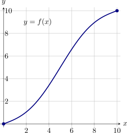
Uma montanha-russa de brinquedo foi projetada de modo que o trilho tem a forma
do gráfico de \(f(x) = x - \sin \left (\frac {\pi x}{5}\right )\), onde \(x\) e \(f(x)\) são medidos em polegadas.
A taxa de variação média da altitude da montanha-russa no intervalo \([0,10]\) é
\(\class{xm-answer}{\cssId{xm-answer-1}{\phantom{\rule{7em}{1.5em}}}}\).
Selecione a melhor interpretação de \(f'(a)\) para \(0<a<10\).
\(f'(a)\) é a altitude em \(a\). \(f'(a)\) é a taxa de
variação média da altitude no intervalo \([0,a]\). \(f'(a)\) é a velocidade de um objeto em \(a\). \(f'(a)\) é a
taxa de variação instantânea da altitude em \(a\). \(f'(a)\) é a inclinação da reta secante que
passa por \((0,0)\) e \((10,10)\).
Como \(f\) é contínuaderivável no intervalo \([0,10]\) e \(f\) é contínuaderivável no intervalo
\((0,10)\), \(f\) satisfaz as hipóteses do teorema do valor médio.
Pelo teorema do valor médio, existe \(c\) em \((0,10)\) tal que \(f'(c) = 1\). Na verdade, isso acontece duas
vezes: quando \(c_1=\class{xm-answer}{\cssId{xm-answer-2}{\phantom{\rule{7em}{1.5em}}}}\) e quando \(c_2=\class{xm-answer}{\cssId{xm-answer-3}{\phantom{\rule{7em}{1.5em}}}}\) (suponha \(c_1<c_2\)).
O ponto mais íngreme da montanha-russa é \(\left (\class{xm-answer}{\cssId{xm-answer-4}{\phantom{\rule{7em}{1.5em}}}},\class{xm-answer}{\cssId{xm-answer-5}{\phantom{\rule{7em}{1.5em}}}}\right )\). (Dica: maximize \(f'(x)\) em \((0,10)\).)
A aproximação linear, \(L\), de \(f\) em \(a=5\) é \[ L(x) = \class{xm-answer}{\cssId{xm-answer-6}{\phantom{\rule{7em}{1.5em}}}}. \]
Usando essa aproximação linear, estimamos que \(f(7)\) é aproximadamente \[ f(7) \approx \class{xm-answer}{\cssId{xm-answer-7}{\phantom{\rule{7em}{1.5em}}}}. \] Essa
estimativa é uma estimativa por excessoestimativa por falta porque \(f\) tem concavidade para cimaconcavidade para baixo entre 5 e 7.
Quando \(x\) varia de \(x=5\) até \(x+\Delta x=7\), a variação de \(f\), \(\Delta y\), é \[ \Delta y = \class{xm-answer}{\cssId{xm-answer-8}{\phantom{\rule{7em}{1.5em}}}}. \] Podemos aproximar essa variação pela
diferencial \(\mathrm {d}y\), que é \[ \mathrm {d}y = \class{xm-answer}{\cssId{xm-answer-9}{\phantom{\rule{7em}{1.5em}}}}. \] (Dica: consulte a definição de diferenciais no livro.)