Taxas relacionadas aplicadas

\( \newenvironment {prompt}{}{} \newcommand {\accordion }[0]{} \newcommand {\ungraded }[0]{} \newcommand {\xmDefaultPreamble }[0]{xmPreamble.tex} \newcommand {\xmDefaultPrintstyle }[0]{xmPrintstyle.sty} \newcommand {\todo }[0]{} \newcommand {\oiint }[0]{{\large \bigcirc }\kern -1.56em\iint } \newcommand {\mooculus }[0]{\textsf {\textbf {MOOC}\textnormal {\textsf {ULUS}}}} \newcommand {\tkzTabSlope }[1]{\foreach \x /\y /\z in {#1}{\node [left = 3pt] at (Z\x 1) {\scriptsize $\y $}; \node [right = 3pt] at (Z\x 1) {\scriptsize $\z $}; }} \newcommand {\RR }[0]{\mathbb R} \newcommand {\R }[0]{\mathbb R} \newcommand {\N }[0]{\mathbb N} \newcommand {\Z }[0]{\mathbb Z} \newcommand {\sagemath }[0]{\textsf {SageMath}} \newcommand {\d }[0]{\,d} \newcommand {\l }[0]{\ell } \newcommand {\ddx }[0]{\frac {d}{\d x}} \newcommand {\zeroOverZero }[0]{\ensuremath {\boldsymbol {\tfrac {0}{0}}}} \newcommand {\inftyOverInfty }[0]{\ensuremath {\boldsymbol {\tfrac {\infty }{\infty }}}} \newcommand {\zeroOverInfty }[0]{\ensuremath {\boldsymbol {\tfrac {0}{\infty }}}} \newcommand {\zeroTimesInfty }[0]{\ensuremath {\small \boldsymbol {0\cdot \infty }}} \newcommand {\inftyMinusInfty }[0]{\ensuremath {\small \boldsymbol {\infty - \infty }}} \newcommand {\oneToInfty }[0]{\ensuremath {\boldsymbol {1^\infty }}} \newcommand {\zeroToZero }[0]{\ensuremath {\boldsymbol {0^0}}} \newcommand {\inftyToZero }[0]{\ensuremath {\boldsymbol {\infty ^0}}} \newcommand {\numOverZero }[0]{\ensuremath {\boldsymbol {\tfrac {\#}{0}}}} \newcommand {\dfn }[0]{\textbf } \newcommand {\unit }[0]{\mathop {}\!\mathrm } \newcommand {\eval }[1]{\bigg [ #1 \bigg ]} \newcommand {\seq }[1]{\left ( #1 \right )} \newcommand {\epsilon }[0]{\varepsilon } \newcommand {\phi }[0]{\varphi } \newcommand {\iff }[0]{\Leftrightarrow } \DeclareMathOperator {\arccot }{arccot} \DeclareMathOperator {\arcsec }{arcsec} \DeclareMathOperator {\arccsc }{arccsc} \DeclareMathOperator {\si }{Si} \DeclareMathOperator {\scal }{scal} \DeclareMathOperator {\sign }{sign} \newcommand {\arrowvec }[1]{{\overset {\rightharpoonup }{#1}}} \newcommand {\vec }[1]{{\overset {\boldsymbol {\rightharpoonup }}{\mathbf {#1}}}\hspace {0in}} \newcommand {\point }[1]{\left (#1\right )} \newcommand {\pt }[1]{\mathbf {#1}} \newcommand {\Lim }[2]{\lim _{\point {#1} \to \point {#2}}} \DeclareMathOperator {\proj }{\mathbf {proj}} \newcommand {\veci }[0]{{\boldsymbol {\hat {\imath }}}} \newcommand {\vecj }[0]{{\boldsymbol {\hat {\jmath }}}} \newcommand {\veck }[0]{{\boldsymbol {\hat {k}}}} \newcommand {\vecl }[0]{\vec {\boldsymbol {\l }}} \newcommand {\uvec }[1]{\mathbf {\hat {#1}}} \newcommand {\utan }[0]{\mathbf {\hat {t}}} \newcommand {\unormal }[0]{\mathbf {\hat {n}}} \newcommand {\ubinormal }[0]{\mathbf {\hat {b}}} \newcommand {\dotp }[0]{\bullet } \newcommand {\cross }[0]{\boldsymbol \times } \newcommand {\grad }[0]{\boldsymbol \nabla } \newcommand {\divergence }[0]{\grad \dotp } \newcommand {\curl }[0]{\grad \cross } \newcommand {\lto }[0]{\mathop {\longrightarrow \,}\limits } \newcommand {\bar }[0]{\overline } \newcommand {\surfaceColor }[0]{violet} \newcommand {\surfaceColorTwo }[0]{redyellow} \newcommand {\sliceColor }[0]{greenyellow} \newcommand {\vector }[1]{\left \langle #1\right \rangle } \newcommand {\sectionOutcomes }[0]{} \newcommand {\VerbMathToks }[2]{\alteqtoks {\begin {#2} #1 \end {#2}}} \newcommand {\DeclareMicrotypeVariants }[1]{} \newcommand {\DeclareMicrotypeAlias }[2]{} \newcommand {\LoadMicrotypeFile }[1]{} \newcommand {\DeclareMicrotypeFilePrefix }[1]{} \newcommand {\DeclareMicrotypeBabelHook }[2]{} \newcommand {\microtypesetup }[1]{} \newcommand {\microtypecontext }[1]{} \newcommand {\textmicrotypecontext }[2]{#2} \newcommand {\leftprotrusion }[1]{#1} \newcommand {\rightprotrusion }[1]{#1} \newcommand {\noprotrusionifhmode }[0]{} \newcommand {\lsstyle }[0]{} \newcommand {\lslig }[1]{#1} \newcommand {\maketitle }[0]{} \newcommand {\problem }[0]{ } \newcommand {\exercise }[0]{ } \newcommand {\question }[0]{ } \newcommand {\exploration }[0]{ } \newcommand {\dialogue }[0]{\begin {description}} \newcommand {\GetTranslation }[1]{#1} \)

Resolvemos problemas de taxas relacionadas em contexto.

Agora estamos prontos para resolver problemas de taxas relacionadas em contexto. Assim como antes, vamos seguir essencialmente o mesmo plano de ataque em cada problema.

Introduza variáveis, identifique a taxa dada e a taxa desconhecida.: Atribua uma variável a cada quantidade que varia no tempo.
Faça um desenho.: Se possível, faça um desenho esquemático com todas as informações relevantes.
Encontre as equações.: Escreva equações que relacionem todas as variáveis relevantes.
Derive em relação a t.: Aqui, frequentemente usaremos derivação implícita e obteremos uma equação que relaciona a taxa dada e a taxa desconhecida.
Substitua e resolva.: Calcule cada quantidade no instante relevante e resolva para a taxa desconhecida.

1 Fórmulas

No nosso próximo problema, vamos esticar e achatar uma massa de pizza em forma de cilindro.

Uma massa de pizza aberta à mão começa como uma bola de massa com volume de $400\pi \, \text {cm}^3$. Primeiro, o cozinheiro estica a massa até a forma de um cilindro de raio $12$ cm. Em seguida, o cozinheiro lança a massa para o alto.

Se, durante o lançamento, a massa mantém a forma de um cilindro e o raio está aumentando a uma taxa de $15$ cm/min, com que rapidez a sua espessura está variando quando o raio é $20$ cm?

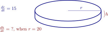
Primeiro, introduzimos as variáveis $V$, $r$ e $h$, que denotam o volume, o raio e a espessura da pizza, nessa ordem. Identificamos a taxa dada $\frac {dr}{dt}=15$ cm/min e a taxa desconhecida $\frac {dh}{dt}$, quando $r=20$.

Em seguida, fazemos um desenho. Observe que a nossa massa de pizza tem a forma de um cilindro.

Agora precisamos encontrar equações. Lembre-se da fórmula do volume do cilindro, $V=\pi \cdot r^2\cdot h$, observe que $V=400\pi \, \text {cm}^3$ e escreva \[ 400\pi = \pi \cdot r^2 \cdot h, \] o que se simplifica imediatamente para \[ 400 = r^2 \cdot h. \] Como tanto $r$ quanto $h$ são funções do tempo, agora derivamos ambos os lados da equação usando derivação implícita,

\[ 0 = 2\cdot r \cdot \frac {dr}{dt} \cdot h+ r^2 \cdot \frac {dh}{dt}. \] Agora vamos calcular todas as quantidades no instante em que $r=20$. Mas, primeiro, temos que calcular $h$ nesse momento. Como \[ 400 = 20^2 \cdot h , \] segue que $h=1$, quando $r=20$. Agora estamos prontos para resolver.

\[ 0 = 2\cdot 20 \cdot 15 \cdot 1 + 20^2 \cdot \frac {dh}{dt} \] \[ \frac {-2\cdot 20 \cdot 15 \cdot 1}{20^2} = \frac {dh}{dt} \] Portanto, quando $r=20$,

\[ \frac {dh}{dt} = -1.5. \] Logo, a espessura da massa está variando a uma taxa de $\class{xm-given}{-1.5}$ cm/min quando $r=20$ cm.

No nosso próximo exemplo, consideramos uma bola de neve derretendo.

Considere uma bola de neve derretendo. Vamos supor que a taxa com que a bola de neve derrete é proporcional à sua área de superfície. Mostre que o raio da bola de neve está variando a uma taxa constante.

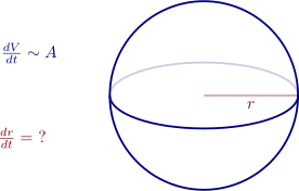
Primeiro, introduzimos as variáveis $V$, $r$ e $A$, que denotam o volume, o raio e a área de superfície da bola de neve, nessa ordem. Em seguida, identificamos a taxa dada $\frac {dV}{dt}$ e a taxa desconhecida $\frac {dr}{dt}$, a taxa a ser determinada. Este problema é um pouco incomum, porque “a taxa dada” não é dada explicitamente. Vamos lidar com essa questão mais abaixo. Em seguida, fazemos um desenho.

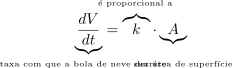
Para encontrar equações que relacionem todas as variáveis relevantes, lembramos as fórmulas do volume e da área de superfície da esfera, \[ (1) \hspace {0.1in} V =\frac {4}{3} \cdot \pi \cdot r^3 \qquad \text {e}\qquad (2) \hspace {0.1in} A = 4 \pi \cdot r^2. \] Agora, as palavras-chave são “a taxa com que a bola de neve derrete (a taxa dada) é proporcional à sua área de superfície”. Disso obtemos a seguinte equação:

Precisamos calcular $\frac {dV}{dt}$. Como $r$ é uma função de $t$, derivamos ambos os lados da equação $(1)$. Assim, \[ \frac {dV}{dt} = 4\cdot \pi \cdot r^2 \cdot \frac {dr}{dt}. \] Por outro lado, \[ \frac {dV}{dt} = k\cdot A. \] Portanto, \[ 4\cdot \pi \cdot r^2 \cdot \frac {dr}{dt} = k\underbrace {\cdot 4\cdot \pi \cdot r^2}_{A} . \] Agora, resolvemos para $\frac {dr}{dt}$ e obtemos que \begin{align*} \frac {dr}{dt} &= k.\\ \end{align*}

Logo, o raio está variando a uma taxa constante. Note que, neste exemplo, não tivemos que calcular as quantidades em um instante particular, porque a taxa desconhecida não dependia do tempo.

2 Triângulos retângulos

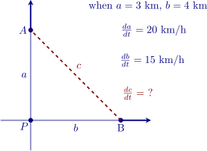
Uma estrada que vai de norte a sul cruza uma estrada que vai de leste a oeste no ponto $P$. O ciclista $A$ está pedalando para o norte pela primeira estrada, e o ciclista $B$ está pedalando para o leste pela segunda estrada. Em um certo instante, o ciclista $A$ está $3$ quilômetros ao norte de $P$ e se deslocando a $20$ km/h, enquanto o ciclista $B$ está $4$ quilômetros a leste de $P$ e se deslocando a $15$ km/h. Com que rapidez a distância entre os dois ciclistas está variando nesse instante?

Primeiro, introduzimos as variáveis $a$, $b$ e $c$, que denotam a distância do ciclista $A$ ao ponto $P$, a distância do ciclista $B$ ao ponto $P$ e a distância entre os dois ciclistas, nessa ordem. Identificamos as taxas dadas $\frac {da}{dt}=20$ km/h, $\frac {db}{dt}=15$ km/h, quando $a=3, b=4$, e a taxa desconhecida $\frac {dc}{dt}$, quando $a=3, b=4$. Agora, fazemos um desenho.

Encontramos equações que relacionam as variáveis $a$, $b$ e $c$. Pelo teorema de Pitágoras, \[ (1)\hspace {0.2in}c^2=a^2+b^2. \] Como $a$, $b$ e $c$ são funções do tempo, derivamos ambos os lados da equação em relação a $t$. \[ (2)\hspace {0.2in}2\cdot c\cdot \frac {dc}{dt}=2\cdot a\cdot \frac {da}{dt}+2\cdot b\cdot \frac {db}{dt}. \] Essa equação vale em algum intervalo de tempo e, em particular, no instante em que $a=3$ e $b=4$. Portanto, nesse instante,

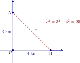
\[ (3)\hspace {0.2in}2\cdot c \cdot \underbrace {\frac {dc}{dt}}_{unknown\hspace {0.015in} rate} =2\cdot 3\cdot \underbrace {20}_ {given\hspace {0.02in} rate}+2\cdot 4 \cdot \underbrace {15}_{given\hspace {0.02in} rate} . \]

Para calcular $c$, a distância entre os ciclistas, no instante em que $a=3$ e $b=4$, fazemos um desenho “tirado” nesse instante.

Pelo teorema de Pitágoras e pelo desenho acima, quando $a=3$, $b=4$, segue que \[ c= \class{xm-given}{5} km. \] Agora podemos calcular todas as quantidades na equação $(3)$ e resolver \[ 2\cdot 5 \cdot \frac {dc}{dt} = 2 \cdot 3\cdot 20 + 2 \cdot 4 \cdot 15. \] Encontramos que $\frac {dc}{dt} = 24$ km/h no momento em que $a=3$, $b=4$.

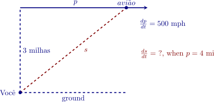
Um avião está voando a uma altitude de $3$ milhas, afastando-se de você em linha reta a $500$ mph . Com que rapidez a distância do avião até você está aumentando no momento em que o avião está sobrevoando um ponto do solo a $4$ milhas de você?

Primeiro, introduzimos as variáveis $p$, a distância que o avião percorreu depois de passar bem acima de você, e $s$, a distância entre você e o avião. A taxa dada é $\frac {dp}{dt}=500$ mph e a taxa desconhecida é $\frac {ds}{dt}$, quando $p=4$. Em seguida, fazemos um desenho.

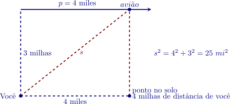
Em seguida, encontramos equações que relacionam as variáveis $p$ e $s$. Pelo teorema de Pitágoras, sabemos que \[ p^2+3^2=s^2. \] Como $p$ e $s$ são funções do tempo, agora derivamos ambos os lados da equação \[ 2\cdot p\cdot \frac {dp}{dt} = 2\cdot s \cdot \frac {ds}{dt}. \] No instante em que $p=4$ mi, obtemos que \[ 2\cdot 4\cdot \underbrace { 500}_{given\hspace {0.02in}rate} = 2\cdot \overbrace {s}^{unknown\hspace {0.02in}value} \cdot \underbrace {\frac {ds}{dt}}_{unknown\hspace {0.02in}rate} . \] Isso implica que $s$ precisa ser calculado no instante em que $p=4$. Para fazer isso, vamos desenhar a figura no instante dado, quando $p=4$ mi.

Assim, $s=\class{xm-given}{5}$. Juntando todas as informações, obtemos \[ 2(4)(500)=2(5)\frac {ds}{dt} . \] Finalmente, resolvemos: $\frac {ds}{dt}=\class{xm-given}{400}$ mph, no momento em que $p=4$ milhas.

3 Taxas angulares

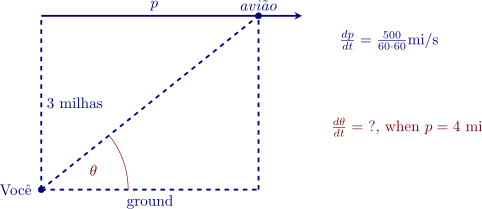
Um avião está voando a uma altitude de $3$ milhas, afastando-se de você em linha reta a $500$ mph . Seja $\theta $ o ângulo de elevação do avião, isto é, o ângulo entre o solo e a sua linha de visada até o avião. Com que rapidez o ângulo $\theta $ está variando no momento em que o avião está sobrevoando um ponto do solo a $4$ milhas de você?

Primeiro, introduzimos uma variável $p$, a distância que o avião percorreu depois de passar bem acima de você. Assim, a taxa dada é $\frac {dp}{dt}=500$ mph e a taxa desconhecida (relacionada) é $\frac {d\theta }{dt}$, no instante em que $p=4$ milhas. Essa taxa deve ser medida em rad/s. Portanto, temos que converter as unidades da taxa dada, mph, para mi/s: $\frac {dp}{dt}=500$mph$=\frac {500}{60\cdot 60}$ mi/s.
Em seguida, fazemos um desenho.

Agora encontramos uma equação que relaciona as variáveis $p$ e $\theta $. Pelo desenho, podemos ver que \[ \tan {\theta }=\frac {3}{p}. \] Como $p$ e $\theta $ são ambas funções do tempo, agora derivamos ambos os lados da equação. Escrevemos \[ \sec ^{2}{\theta }\cdot \frac {d\theta }{dt} = -\frac {3}{p^2}\cdot \frac {dp}{dt}. \] A equação acima vale em algum intervalo de tempo. Em particular, ela é verdadeira quando $p=4$. Portanto, quando $p=4$, \[ \overbrace {\sec ^{2}{\theta }}^{unknown\hspace {0.02in}value}\cdot \underbrace {\frac {d\theta }{dt} }_{unknown\hspace {0.02in}rate} = -\frac {3}{4^2}\cdot \underbrace { \frac {500}{3600}}_{given\hspace {0.02in}rate}. \] Isso implica que temos que calcular o valor desconhecido, $\sec ^{2}{\theta }$, quando $p=4$. 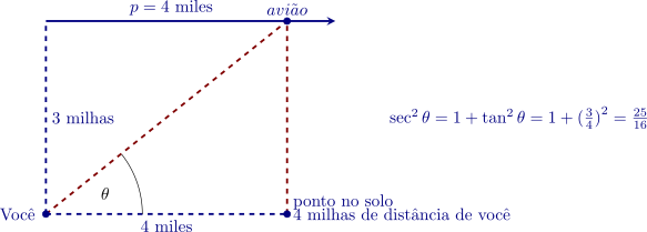Para isso, desenhamos e rotulamos a figura no instante em que $p=4$ mi.

Assim, no momento em que $p=4$ milhas, \[ \sec ^2{\theta }=1+\Bigr (\frac {3}{4}\Bigl )^2=\frac {25}{16}. \] Agora, substituindo todos os valores conhecidos na equação acima, obtemos \[ \frac {25}{16}\cdot \frac {d\theta }{dt}= -\frac {3}{16}\cdot \frac {500}{3600}. \] Resolvemos para $\frac {d\theta }{dt}$, quando $p=4$, e obtemos que \[ \frac {d\theta }{dt} = -\frac {1}{60} rad/s. \]

4 Triângulos semelhantes

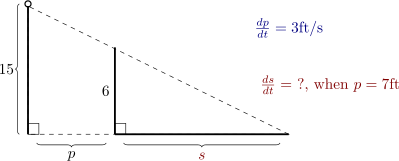
É noite. Uma pessoa de $6$ pés de altura está se afastando de um poste de luz a uma taxa de $3$ pés por segundo. O poste de luz tem $15$ pés de altura. A pessoa projeta uma sombra no chão à sua frente. Com que rapidez o comprimento da sombra está crescendo quando a pessoa está a $7$ pés do poste de luz?

Primeiro, introduzimos duas variáveis: $p$, a distância da pessoa ao poste, e $s$, o comprimento da sombra. A taxa dada é $\frac {dp}{dt}=3$ pés/s e a taxa desconhecida (relacionada) é $\frac {ds}{dt}$ no momento em que $p=7$ pés. Em seguida, fazemos um desenho.

Agora encontramos equações que relacionam as variáveis $p$ e $s$. Usamos o fato de que temos triângulos semelhantes para escrever: \begin{align*} \frac {s+p}{15} &= \frac {s}{\class{xm-given}{6}},\\ 6\cdot s + 6 \cdot p &= 15\cdot s,\\ 6\cdot p &=9\cdot s,\\ 2\cdot p &=3 \cdot s. \end{align*}

Como $p$ e $s$ são ambas funções do tempo, derivamos ambos os lados da equação acima. Usamos derivação implícita e escrevemos \[ 2\cdot \frac {dp}{dt} =3 \cdot \frac {ds}{dt} \] Neste ponto, calculamos todas as quantidades no instante em que $p=7$ pés \[ 2\cdot \cancel {3} = \cancel {3} \cdot \frac {ds}{dt}. \] Agora resolvemos para $\frac {ds}{dt}$ e obtemos que $\frac {ds}{dt}= \class{xm-given}{2}$, quando $p=7$ pés.

Portanto, a sombra está crescendo a uma taxa de $2$ pés/s quando a pessoa está a $7$ pés do poste.

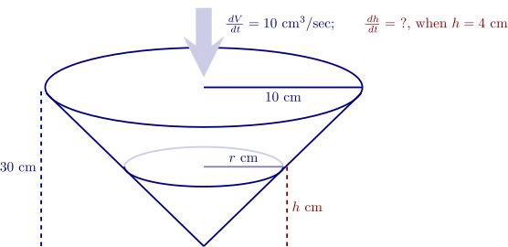
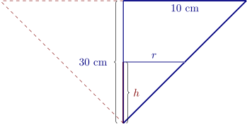
Despeja-se água em um recipiente cônico a uma taxa de 10 cm${}^3$/s. O cone aponta diretamente para baixo e tem altura de 30 cm e raio da base de 10 cm. Com que rapidez o nível da água está subindo quando a água tem 4 cm de profundidade?

Primeiro, introduzimos várias variáveis. Seja $V$ o volume de água no recipiente, seja $r$ o raio da superfície circular da água e seja $h$ a profundidade da água no recipiente. A taxa dada é $\frac {dV}{dt}=10$ $cm^3/s$, e a taxa desconhecida é $\frac {dh}{dt}$, no momento em que $h=4$ cm. Agora, fazemos um desenho.

Observe que não houve nenhuma tentativa de fazer este desenho em escala; em vez disso, queremos que todas as informações relevantes estejam disponíveis para o matemático.

Agora encontramos equações que relacionam todas as variáveis. Observe que a água no recipiente assume a forma do recipiente. Neste exemplo, a forma é um cone. Portanto, usamos a fórmula do volume de um cone \[ V = \frac {\pi }{3} r^2 h. \] Vamos desenhar uma seção transversal do cone.

Observe um triângulo retângulo grande e um triângulo retângulo menor dentro do grande. Esses dois triângulos retângulos são semelhantes, porque seus ângulos correspondentes são iguais. Como as razões entre lados correspondentes de triângulos semelhantes são iguais, obtemos \[ \frac {r}{h}=\frac {10}{30} \qquad \text {logo}\qquad r=\frac {h}{\class{xm-given}{3} }. \] Neste ponto, poderíamos derivar ambos os lados de cada equação, mas podemos adotar uma abordagem mais simples, combinando essas duas equações e expressando $V$ em termos de $h$.

PERGUNTA: Por que é mais conveniente expressar $V$ em termos de $h$ do que em termos de $r$?

Portanto, \[ V = \frac {\pi }{3}\overbrace { \Bigl (\frac {h}{3}\Bigr )^2}^{r^2} h, \] e \[ V = \frac {\pi }{27} \cdot h^3. \] Agora, derivamos em relação a $t$. \[ \dd [V]{t} = \frac {\pi }{27} \cdot 3\cdot h^2\cdot \frac {dh}{dt}. \] Essa equação vale em algum intervalo de tempo. Em particular, a equação é verdadeira no instante em que $h=4$ cm. Agora calculamos todas as quantidades nesse instante. \[ 10 = \frac {\pi }{27} \cdot 3\cdot 4^2\cdot \frac {dh}{dt}. \] Assim, no instante em que a água no recipiente tem $4$ cm de profundidade, o nível da água está subindo a uma taxa de $\frac {45}{8\pi }$ cm/s.