\(
\newenvironment {prompt}{}{}
\newcommand {\accordion }[0]{}
\newcommand {\ungraded }[0]{}
\newcommand {\xmDefaultPreamble }[0]{xmPreamble.tex}
\newcommand {\xmDefaultPrintstyle }[0]{xmPrintstyle.sty}
\newcommand {\todo }[0]{}
\newcommand {\oiint }[0]{{\large \bigcirc }\kern -1.56em\iint }
\newcommand {\mooculus }[0]{\textsf {\textbf {MOOC}\textnormal {\textsf {ULUS}}}}
\newcommand {\tkzTabSlope }[1]{\foreach \x /\y /\z in {#1}{\node [left = 3pt] at (Z\x 1) {\scriptsize $\y $}; \node [right = 3pt] at (Z\x 1) {\scriptsize $\z $}; }}
\newcommand {\RR }[0]{\mathbb R}
\newcommand {\R }[0]{\mathbb R}
\newcommand {\N }[0]{\mathbb N}
\newcommand {\Z }[0]{\mathbb Z}
\newcommand {\sagemath }[0]{\textsf {SageMath}}
\newcommand {\d }[0]{\,d}
\newcommand {\l }[0]{\ell }
\newcommand {\ddx }[0]{\frac {d}{\d x}}
\newcommand {\zeroOverZero }[0]{\ensuremath {\boldsymbol {\tfrac {0}{0}}}}
\newcommand {\inftyOverInfty }[0]{\ensuremath {\boldsymbol {\tfrac {\infty }{\infty }}}}
\newcommand {\zeroOverInfty }[0]{\ensuremath {\boldsymbol {\tfrac {0}{\infty }}}}
\newcommand {\zeroTimesInfty }[0]{\ensuremath {\small \boldsymbol {0\cdot \infty }}}
\newcommand {\inftyMinusInfty }[0]{\ensuremath {\small \boldsymbol {\infty - \infty }}}
\newcommand {\oneToInfty }[0]{\ensuremath {\boldsymbol {1^\infty }}}
\newcommand {\zeroToZero }[0]{\ensuremath {\boldsymbol {0^0}}}
\newcommand {\inftyToZero }[0]{\ensuremath {\boldsymbol {\infty ^0}}}
\newcommand {\numOverZero }[0]{\ensuremath {\boldsymbol {\tfrac {\#}{0}}}}
\newcommand {\dfn }[0]{\textbf }
\newcommand {\unit }[0]{\mathop {}\!\mathrm }
\newcommand {\eval }[1]{\bigg [ #1 \bigg ]}
\newcommand {\seq }[1]{\left ( #1 \right )}
\newcommand {\epsilon }[0]{\varepsilon }
\newcommand {\phi }[0]{\varphi }
\newcommand {\iff }[0]{\Leftrightarrow }
\DeclareMathOperator {\arccot }{arccot}
\DeclareMathOperator {\arcsec }{arcsec}
\DeclareMathOperator {\arccsc }{arccsc}
\DeclareMathOperator {\si }{Si}
\DeclareMathOperator {\scal }{scal}
\DeclareMathOperator {\sign }{sign}
\newcommand {\arrowvec }[1]{{\overset {\rightharpoonup }{#1}}}
\newcommand {\vec }[1]{{\overset {\boldsymbol {\rightharpoonup }}{\mathbf {#1}}}\hspace {0in}}
\newcommand {\point }[1]{\left (#1\right )}
\newcommand {\pt }[1]{\mathbf {#1}}
\newcommand {\Lim }[2]{\lim _{\point {#1} \to \point {#2}}}
\DeclareMathOperator {\proj }{\mathbf {proj}}
\newcommand {\veci }[0]{{\boldsymbol {\hat {\imath }}}}
\newcommand {\vecj }[0]{{\boldsymbol {\hat {\jmath }}}}
\newcommand {\veck }[0]{{\boldsymbol {\hat {k}}}}
\newcommand {\vecl }[0]{\vec {\boldsymbol {\l }}}
\newcommand {\uvec }[1]{\mathbf {\hat {#1}}}
\newcommand {\utan }[0]{\mathbf {\hat {t}}}
\newcommand {\unormal }[0]{\mathbf {\hat {n}}}
\newcommand {\ubinormal }[0]{\mathbf {\hat {b}}}
\newcommand {\dotp }[0]{\bullet }
\newcommand {\cross }[0]{\boldsymbol \times }
\newcommand {\grad }[0]{\boldsymbol \nabla }
\newcommand {\divergence }[0]{\grad \dotp }
\newcommand {\curl }[0]{\grad \cross }
\newcommand {\lto }[0]{\mathop {\longrightarrow \,}\limits }
\newcommand {\bar }[0]{\overline }
\newcommand {\surfaceColor }[0]{violet}
\newcommand {\surfaceColorTwo }[0]{redyellow}
\newcommand {\sliceColor }[0]{greenyellow}
\newcommand {\vector }[1]{\left \langle #1\right \rangle }
\newcommand {\sectionOutcomes }[0]{}
\newcommand {\VerbMathToks }[2]{\alteqtoks {\begin {#2} #1 \end {#2}}}
\newcommand {\DeclareMicrotypeVariants }[1]{}
\newcommand {\DeclareMicrotypeAlias }[2]{}
\newcommand {\LoadMicrotypeFile }[1]{}
\newcommand {\DeclareMicrotypeFilePrefix }[1]{}
\newcommand {\DeclareMicrotypeBabelHook }[2]{}
\newcommand {\microtypesetup }[1]{}
\newcommand {\microtypecontext }[1]{}
\newcommand {\textmicrotypecontext }[2]{#2}
\newcommand {\leftprotrusion }[1]{#1}
\newcommand {\rightprotrusion }[1]{#1}
\newcommand {\noprotrusionifhmode }[0]{}
\newcommand {\lsstyle }[0]{}
\newcommand {\lslig }[1]{#1}
\newcommand {\maketitle }[0]{}
\newcommand {\problem }[0]{ }
\newcommand {\exercise }[0]{ }
\newcommand {\question }[0]{ }
\newcommand {\exploration }[0]{ }
\newcommand {\dialogue }[0]{\begin {description}}
\newcommand {\GetTranslation }[1]{#1}
\)
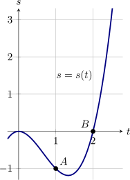
Seja \(s(t) = t^3-2t^2\). O gráfico de \(s\) é dado abaixo.
Os pontos \(A\) e \(B\) são dois pontos no gráfico de \(s\). \[ A=\left (1,\class{xm-answer}{\cssId{xm-answer-1}{\phantom{\rule{7em}{1.5em}}}}\right )\quad B=\left (2,\class{xm-answer}{\cssId{xm-answer-2}{\phantom{\rule{7em}{1.5em}}}}\right ) \]
A inclinação da reta secante que passa pelos pontos \(A\) e \(B\) é \[ m_{\text {sec}}=\class{xm-answer}{\cssId{xm-answer-3}{\phantom{\rule{7em}{1.5em}}}}. \]
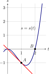
A reta tangente ao gráfico de \(s\) no ponto \(A\) é mostrada acima. Observando essa reta
com atenção, podemos aproximar sua inclinação por \[ m_{\text {tan}}\approx \class{xm-answer}{\cssId{xm-answer-4}{\phantom{\rule{7em}{1.5em}}}}. \]
Em termos da função \(s\), o limite que teríamos de calcular para obter a inclinação da
reta tangente a \(s\) em \(t=1\) é \[ m_{\text {tan}} = \lim _{t\to 1}\frac {s(\class{xm-answer}{\cssId{xm-answer-5}{\phantom{\rule{7em}{1.5em}}}})-s(1)}{\class{xm-answer}{\cssId{xm-answer-6}{\phantom{\rule{7em}{1.5em}}}}}. \] Quando substituímos a fórmula de \(s\), obtemos o seguinte
limite, escrito em termos de \(t\): \[ m_{\text {tan}} = \lim _{t\to 1}\frac {\class{xm-answer}{\cssId{xm-answer-7}{\phantom{\rule{7em}{1.5em}}}}}{\class{xm-answer}{\cssId{xm-answer-8}{\phantom{\rule{7em}{1.5em}}}}}. \]
Suponha que a função \(s(t) = t^3-2t^2\) represente a posição, no instante \(t\), de um objeto que se move
ao longo de uma reta, em que \(s\) é medida em pés e \(t\) é medido em segundos. A
velocidade média do objeto no intervalo de tempo \([1,2]\) é \[ v_{\text {méd}} = \class{xm-answer}{\cssId{xm-answer-9}{\phantom{\rule{7em}{1.5em}}}} ft/s. \]
Complete a tabela a seguir com as velocidades médias apropriadas (em \(ft/s\)).
\[ \begin{array}{|c|c|} \hline \text {Time interval} & \text {Average velocity} \\\hline \hline [1,2] & \class{xm-answer}{\cssId{xm-answer-10}{\phantom{\rule{7em}{1.5em}}}} \\\hline [1,1.5] & \class{xm-answer}{\cssId{xm-answer-11}{\phantom{\rule{7em}{1.5em}}}} \\\hline [1,1.1] & \class{xm-answer}{\cssId{xm-answer-12}{\phantom{\rule{7em}{1.5em}}}} \\\hline [0.5,1] & \class{xm-answer}{\cssId{xm-answer-13}{\phantom{\rule{7em}{1.5em}}}} \\\hline [0.9,1] & \class{xm-answer}{\cssId{xm-answer-14}{\phantom{\rule{7em}{1.5em}}}} \\\hline \end{array} \]
Com base nos valores acima, uma conjectura razoável para a velocidade instantânea
do objeto em \(t=1\) é \[ v_{\text {inst}}\approx {\class{xm-answer}{\cssId{xm-answer-15}{\phantom{\rule{7em}{1.5em}}}}} ft/s. \]
Em termos da função \(s\), o limite que teríamos de calcular para obter a velocidade
instantânea do objeto em \(t=1\) é \[ v_{\text {inst}} = \lim _{t\to 1}\frac {s(\class{xm-answer}{\cssId{xm-answer-16}{\phantom{\rule{7em}{1.5em}}}})-s(1)}{\class{xm-answer}{\cssId{xm-answer-17}{\phantom{\rule{7em}{1.5em}}}}}. \] Observe que essa é exatamente a mesma expressão que
precisaríamos calcular para obter a inclinação da reta tangente ao gráfico de \(s(t)\) em
\(t=1\).